[abstract]

• propose a framewalk to estimate graphlet statistics of “any size”
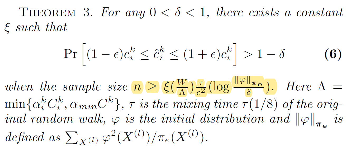
• analytic bound of the sample size (Chernoff-Hoeffding) to guarantee convergence

[1. introduction]

• estimating graphlets is more complicated than estimating local structures (e.g. degree distribution)

[1.1 Related Works and Existing Problems]

1. memory-based graphs : wedge sampling
   • need access to the whole graph
2. streaming graphs
   • access each edge at least once
3. restricted accessed graphs : SRW, PSRW, MSS
   • random walk based methods

[1.2 Our contributions]

1. novel framework
   • no assumption on the graph structures
   • propose a new and general frameworks which subsumes PSRW
2. efficient optimization techniques
   • corresponding state sampling (CSS)
   • non-backtracking random walk

[2.1 Notations and Definitions]

• $G^{(d)}=(H^{(d)}, R^{(d)})$: d-node subgraph relationship graph
• $H^{(d)}$: the set of all d-node connected induced subgraphs of G
• For $s_i, s_j\in H^{(d)}$, if they share d-1 common nodes in G, there is an edge. Denote the set of these edges as $R^{(d)}$.
• For d=1, define $G^{(1)}=G$ (and the same for H, R)

⇒ constructing $G^{(d)}$ requires compuational cost. no need to construct it using random-walk technique

⇒ The number of distinct graphlets grows exponentially with the numbeer of vertices in the graphlets

⇒ problem definition: estimate “concentration of graphlets”

[2.2 Random walk and Markov Chain]

• A simple random walk (SRW)
  • random walk : a finite and time-reversible Markov chain with state space V
    • ${X_t}$: Markov chain representing the visited nodes of the random walk on G
    • P: transition probability defined as $P(i,j)=1/d_i$ if $(i,j)\in E$ and 0 otherwise.
  • unique stationary distribution $\pi$ where $\pi(v)=d_v/2\abs{E}$ ⇒ correct bias
• Strong Law of Large Numbers (SLLN)

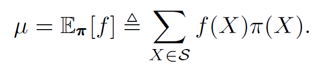
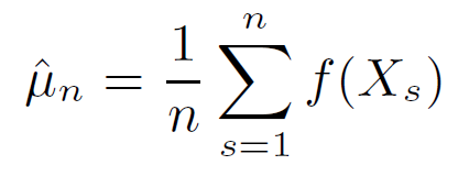
⇒ By SLLN, $\hat{\mu}_n$ converges to $\mu$ .

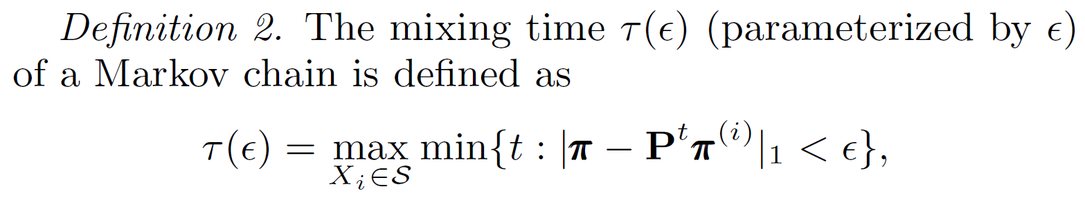
• Mixing time : the numbeer of steps it takes for a random walk to approach its stationary distribution

  

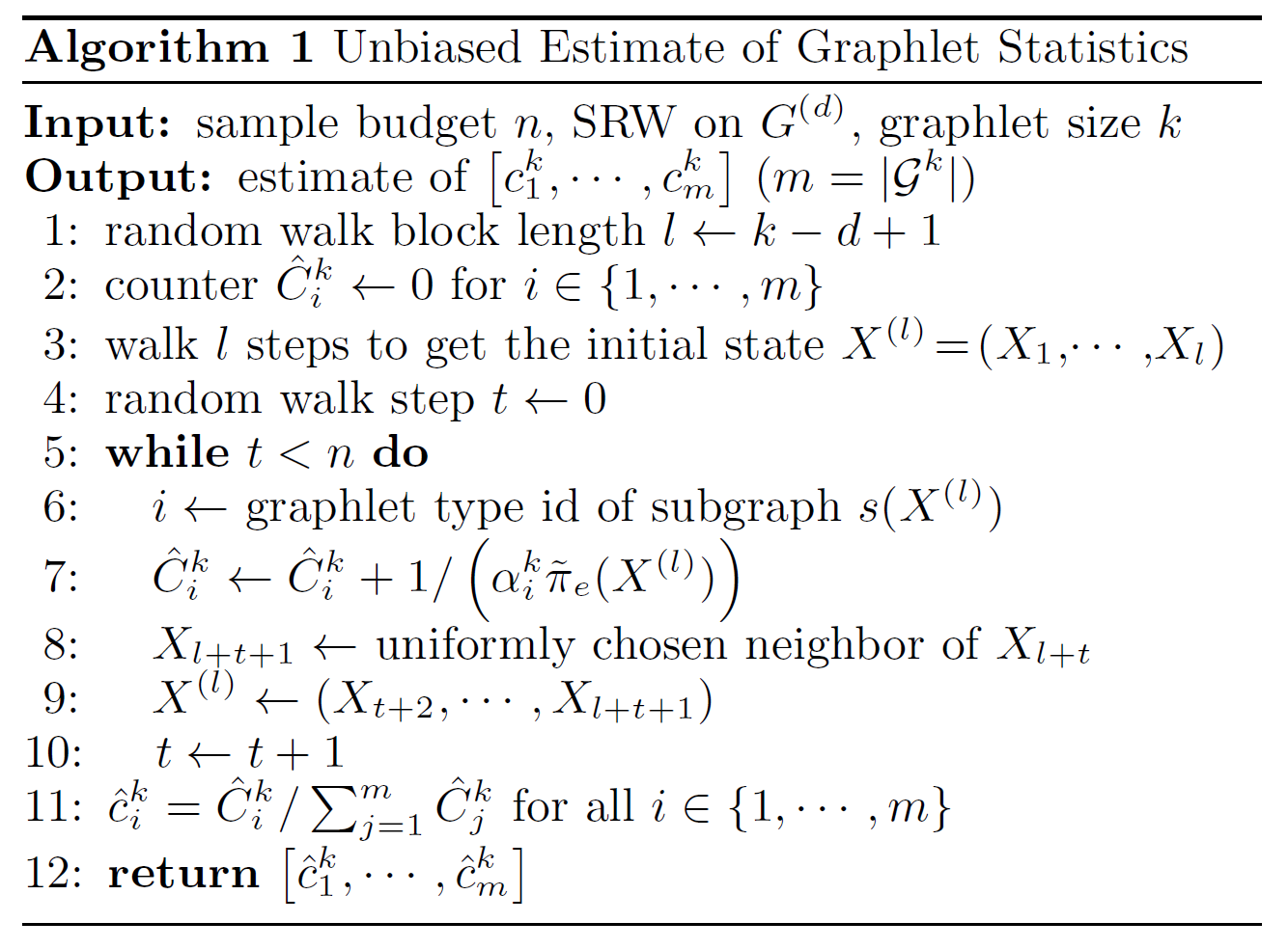
[3.1 Basic Idea]

• d는 hyperparameter로, $G^{(d)}$와 $l=k-d+1$ consecutive steps를 결정
• 각 $X_i (i\geq l)$ 스텝마다 $l-1$ 개의 전 스텝을 기억
• $G^{(d)}$에서 random walk 시행 후 $X^{(l)}=(X_{i-l+1}, \dots, X_i)$로 induced 된 subgraph를 고려
• 만약 induced subgraph의 크기가 k미만이면, 다시 l consecutive step을 찾음

[3.2 Expanded Markov Chain]

• Each $l$ consecutive steps are considered as a state $X^{(l)}=(X_1, \cdots, X_l)$ of the expanded Markov chain
• state space $M^{(l)} = \set{(X_1, \cdots, X_l): X_i\in N, 1\leq i\leq l \text{ s.t. } (X_i, X_{i+1})\in R^{(d)} \;\forall 1\leq i\leq l-1}$ (”expanded” MC)
• define expanded MC for convenience of deriving unbiased estimator
  • bias causes from two aspects
    1. states in the expanded Markov chain do not have eqal stational probabilities
    2. a graphlet samples corresponds to several states

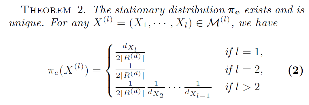
• stationary distribution : $\pi_e$ (stationary distribution of the expandned MC) can be computed by $\pi$ (stationary distribution of the random walk)
• state corresponding coefficient $\alpha_i^k = \abs{C(s)}$ where $C(s)=\set{X^{(l)}:s(X^{(l)})=s, X^{(l)}\in M^{(l)}}$.
• if states in $M^{(l)}$ are uniformly sampled, then the probability of getting a subgraph isomorphic to $g_i^k$ is $\alpha_i^kC_i^k/\abs{M^{(l)}}$.
• $\alpha_i^k$= twice the number of Hamiltonian paths

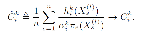
[3.3 Unbiased Estimator]

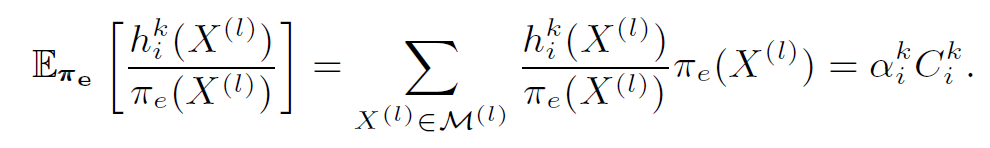
• $h_i^k(X^{(l)})=1{s(X^{(l)})= g_i^k}$.
• $\sum_{X^{(l)}\in M^{(l)}} h_i^k(X^{(l)})=\alpha_i^kC_i^k$.

[4.1 Corresponding State Sampling (CSS)]

• For X=(u, v, w) and Y=(v, w, u), $\pi_e(X)$ might be differerent with $\pi_e(Y)$

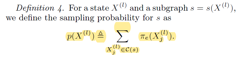
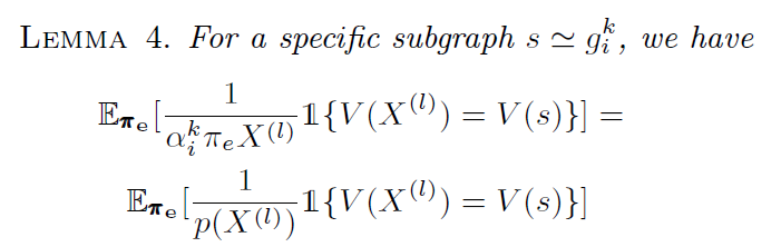
• To solve this issue, we define “sampling probability” $p(X^{(l)})$

  

• If substitue $\pi_e$ on line 7 with p, we also get unbiased estimator

• Vaiance is much more smaller when we use p instead of $\pi_e$

[4.2 Non-backtracking random walk]

• avoid backtracking to the previously visited node
• define augmented space $\Omega=\set{(i,j): i,j\in H^{(d)}, \text{ s.t. }(i,j)\in R^{(d)}}$ and new transition matrix $P’$

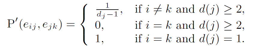
• fact: NB-SRW preserves the stationary distribution of the original random walks