[Abstract]

• introduce a novel graph generative model: Computation Graph Transformer (CGT)
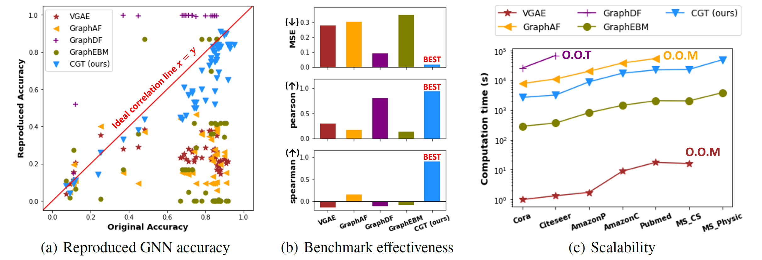
  1. generates effective benchmark graphs on which GNNs show similar task performance as on the source graphs
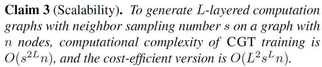
  2. scales to procecss large-scale graphs
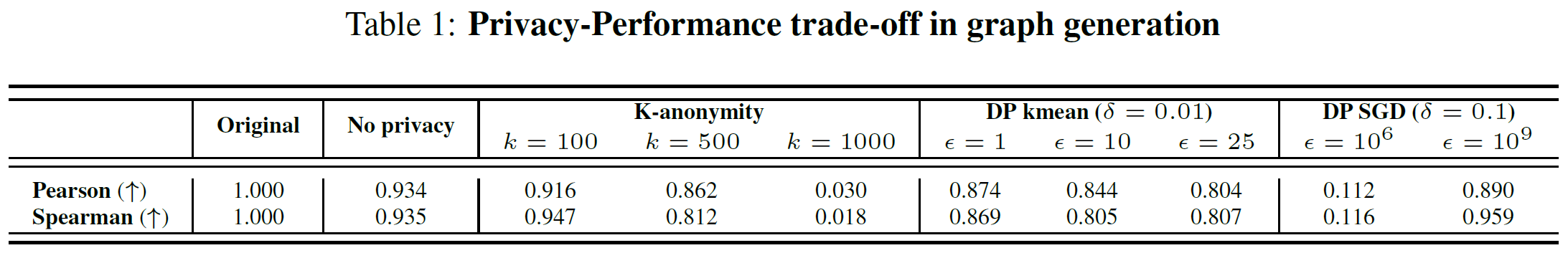
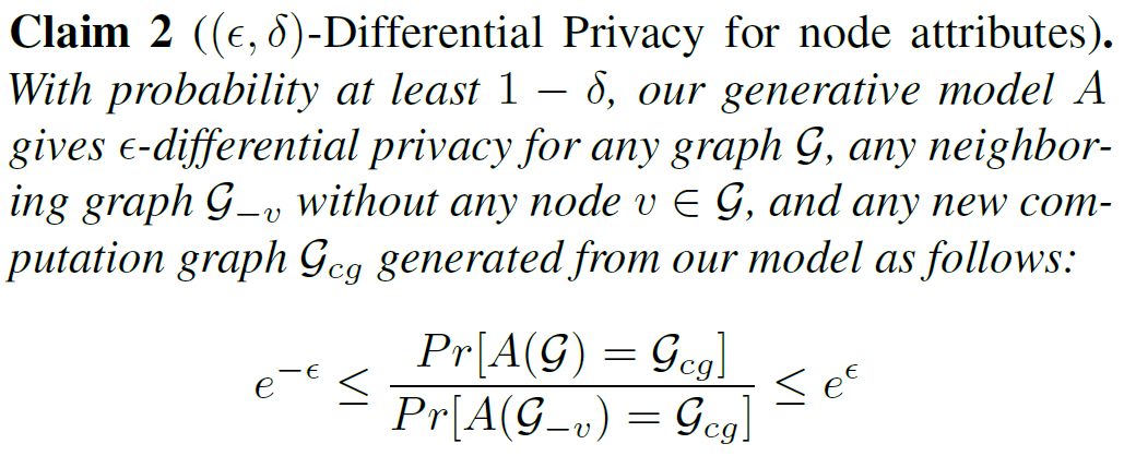
  3. incorporates off-the-shelf privacy modules to guarantee end-user privacy of the generated graph

[1. Introduction]

• graph data: privacy-restricted
• want to overcome the limited access to real-world graph datasets
• goal: generate synthetic graphs that follow its distribution in terms of graph structure, node attributes, and labels (substitues for the original graph)
• problem statement: for a given G=(A, X, Y) (A: adjacency, X: node attributes, Y: node label), generate G’=(A’, X’, Y’) satisfying
  • benchmark effectiveness
    • performance ranking on G’ ~ that of G
  • scalibility
    • linear to a size of graph
  • privacy guarantee

  ⇒ no study fully addressing the problem

• introduce CGT
  • reframe: graph generation problem → discrete-value sequence generation problem
    • learn distirbution of computation graphs rather than whole graph
  • a novel duplicate encoding scheme for computational graphs
  • quantize the feature matrix → discrete value sequence

[2. Related work]

• traditional graph generative models

  ⇒ focus on generating graph structures

• general-purpose deep graph generative models
  • GAN, VAE, RNN
  • evaluation metrics: orbit counts, degree coeffs, clustering coefficients
  • doesn’t consider quality of generated node attributes and labels
• molecule graph generative models

[3. From graph generation to sequence generation]

[3.1 Computation graph sampling in GNN training]

• GNNs extract each node v’s egonet (computation graph) instead of operating on the whole graph
• compute embedding of node v on Gv
• problem reduces to:
  • given a set of computation graphs {Gv=(Av, Xv, Yv): v\in G} sampled from an original graph, we generate a set of computation graphs {G’v=(A’v, X’v, Y’v)}.

[3.2 Duplicate encoding scheme for computation graphs]

• rules of sampling methods
  1. #neighbors sampled for each node is limited to keep computation graphs small
  2. maximum distance from the target node v to sampled nodes is decided by the depth of GNN models

  ⇒ maximum number of neighbors = neighbor sampling number s

  ⇒ maximum number of hops from the target node = depth of computation graphs L

  

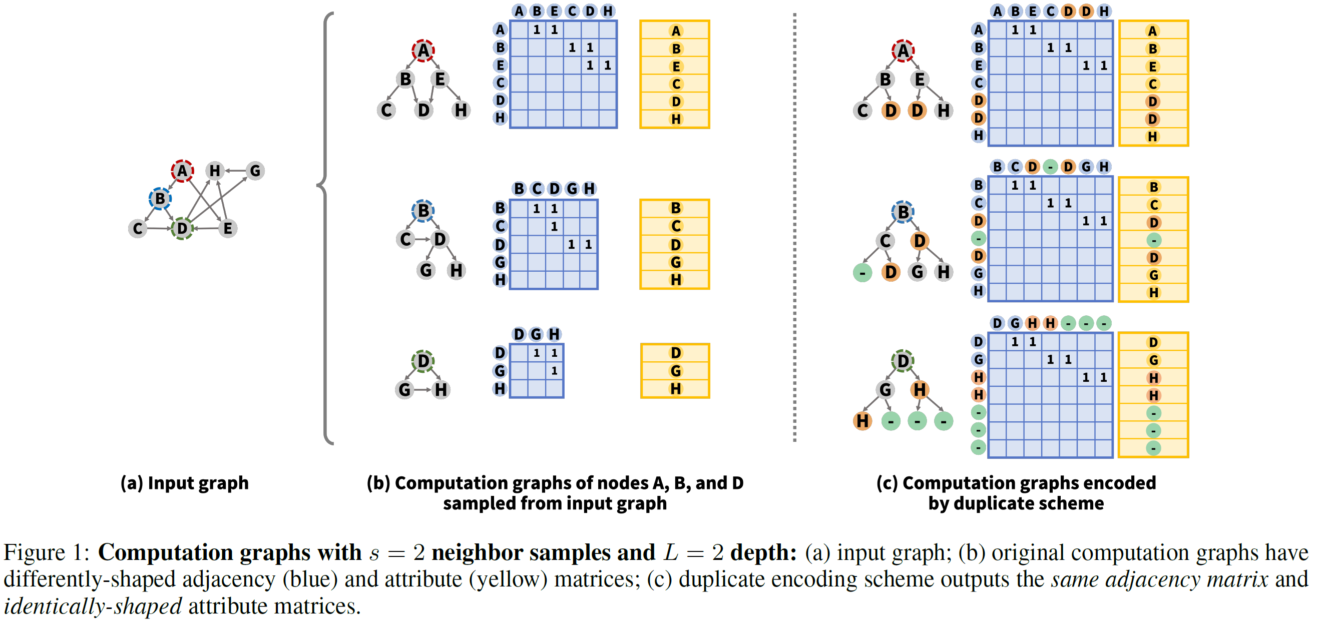
• duplicate encoding scheme
  • fixes the structure of all computation graphs ⇒ L-layered s-nary tree structure
  • let adjacenccy matrix as a constant
  • if deg(v)<s, employ a null node with zero attribute vector, samples it as a padding neighbor
  • when a node has a neighbor sampled by another node, duplicate encoding scheme copies the shared neighbor and provides each copy to parent nodes
  • have to fix the order of nodes (like, breadth-first ordering)

  ⇒ given a set of feature matrix-label pairs of duplicated-encoded computation graphs, we generate a set of feature matrix-label pairs

[3.3 Quantization]

• goal: learn distribution of feature matrices of computation graphs
• method: quantize feature vectors into discrete bins
  • cluster feature vectors in the original graph using k-means
  • map each feature vector to its cluster id
• motivated by
  • privacy benefits
  • ease of modeling

[3.4. End-to-end framework for a benchmark graph generation problem]

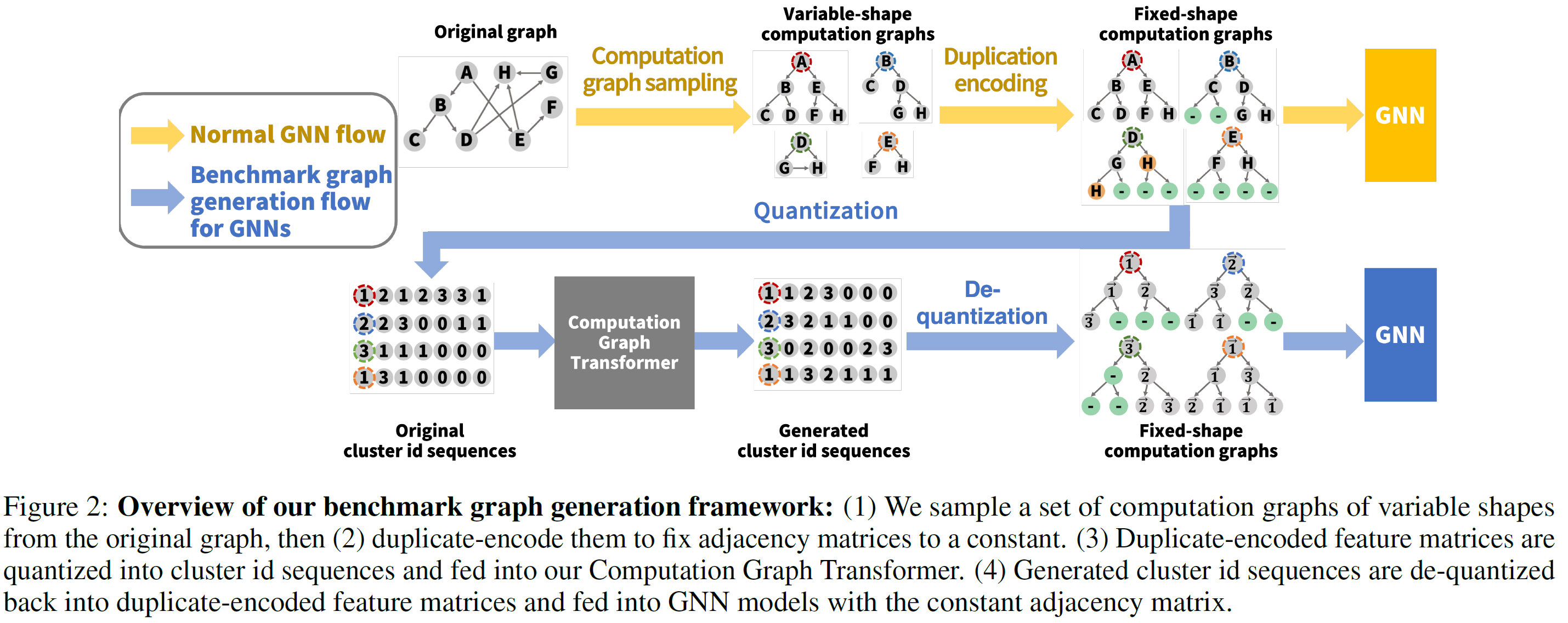
1. sample a set of computation graphs from input graph
2. encode each computation graph using the duplicate encoding scheme to fix adjacency matrix
3. quantize feature vectors to cluster id they belong to
4. hand over a set of pairs to new Transformer architecture
   • generation process: perform through opposite direction

[4. Model]

• encode computational graph structure → sequence generation process with minmal modification to the Transformer architeucture

[4.1 Computation graph transformer (CGT)]

• extend a two-stream self-attention mechanism, XLNet

  • maximize likelihood

    

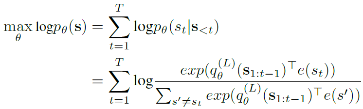
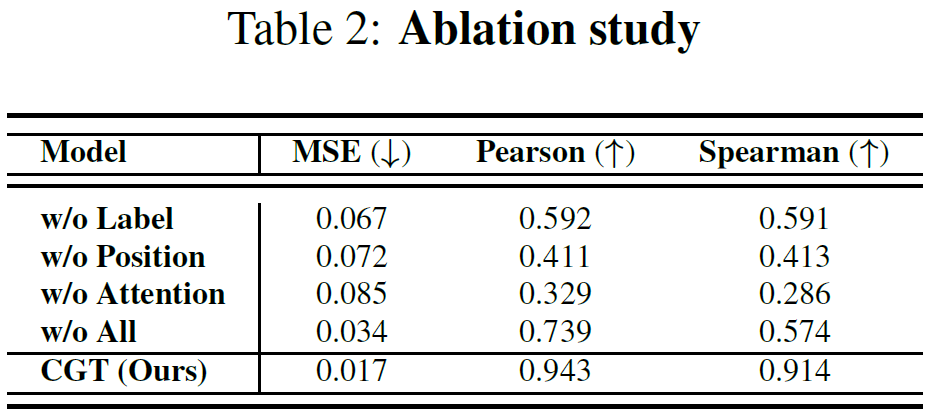
• position embeddings
  • sequence (Fig 3(a)) = flattened computational graph (Fig 3(b))
  • to encode original computational graph structure, provide differnt position embeddings to different layers in the computation graph
  • In figure 3(b), node C, D, F, H located at the 1-st layer have the same position embedding p1

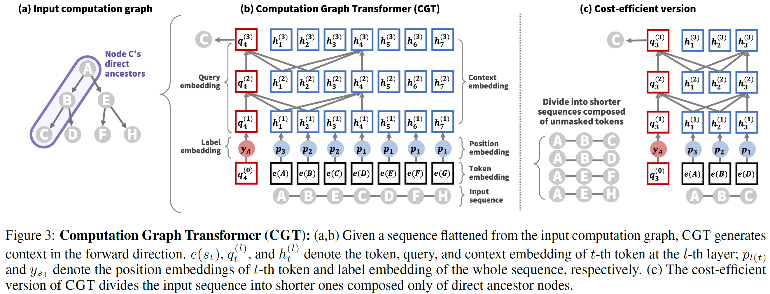
• attention mask
  • $q_t^{(l)}$: query embedding
  • $h_t^{(l)}$: context embedding

  ⇒ two above attend to all context embeddings $h^{(l-1)}_{1:t-1}$ before t

  • each node in the computation graph is sampled based on its parent node, not directly affected by its sibling nodes
  • mask all nodes except direct ancestor nodes in the computation graph
• label conditioning
  • distributions of neighboring nodes are not only affected by each node’s feature information but also by its label
  • without label information, we can’t learn whether a node has feature-wise homogeneous neighbors or feature-wise heterogeneous neighbors but with the same label

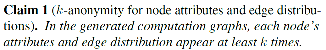
4.2 Theoretical analysis

• provide k-anonymity for node attributes and edge distributions (k-means)

[5. Experiments]

[5.1 Experimental setting]

• Baselines: SOTA graph generative models that learn graph structures with node attribute information